Annotated Example
The best way to get a feel for what Trident can do is to go through an annotated example of its use. This section will walk you through the steps necessary to produce a synthetic spectrum based on simulation data and to view its path through the parent dataset. The following example, available in the source code itself, can be applied to datasets from any of the different simulation codes that Trident and yt support, although it may require some tweaking of parameters for optimal performance. If you want to recreate the following analysis with the exact dataset used, it can be downloaded here.
The basic process for generating a spectrum and overplotting a sightline’s trajectory through the dataset goes in three steps:
Simple LightRay Generation
A LightRay is a 1D object representing the path a ray of
light takes through a simulation volume on its way from some bright background
object to the observer. It records all of the gas fields it intersects along
the way for use in many tasks, including construction of a spectrum.
In order to generate a LightRay from your data, you need to first make sure
that you’ve imported both the yt and Trident packages, and
specify the filename of the dataset from which to extract the light ray:
import yt
import trident
fn = 'enzo_cosmology_plus/RD0009/RD0009'
We need to decide the trajectory that the LightRay will take
through our simulation volume. This arbitrary trajectory is specified with
coordinates in code length units (e.g. [x_start, y_start, z_start] to
[x_end, y_end, z_end]). Probably the simplest trajectory is cutting
diagonally from the origin of the simulation volume to its outermost corner
using the yt domain_left_edge and domain_right_edge attributes. Here
we load the dataset into yt to get access to these attributes:
ds = yt.load(fn)
ray_start = ds.domain_left_edge
ray_end = ds.domain_right_edge
Let’s define what lines or species we want to be added to our final spectrum. In this case, we want to deposit all hydrogen, carbon, nitrogen, oxygen, and magnesium lines to the resulting spectrum from the dataset:
line_list = ['H', 'C', 'N', 'O', 'Mg']
We can now generate the light ray using the make_simple_ray()
function by passing the dataset and the trajectory endpoints to it as well
as telling trident to save the resulting ray dataset to an HDF5 file. We
explicitly instruct trident to pull all necessary fields from the dataset
in order to be able to add the lines from our line_list:
ray = trident.make_simple_ray(ds,
                              start_position=ray_start,
                              end_position=ray_end,
                              data_filename="ray.h5",
                              lines=line_list)
The resulting ray is a LightRay object, consisting of a series
of arrays representing the different fields it probes in the original dataset along
its length. Each element in the arrays represents a different resolution element
along the path of the ray. The ray also possesses some special fields not originally
present in the original dataset:
('gas', l')Location along the LightRay length from 0 to 1.
('gas', 'dl')Pathlength of resolution element (not a true pathlength for particle-based codes)
('gas', 'redshift')Cosmological redshift of resolution element
('gas', 'redshift_dopp')Doppler redshift of resolution element
('gas', 'redshift_eff')Effective redshift (combined cosmological and Doppler)
Like any dataset, you can see what fields are present on the ray by examining its
derived_field_list (e.g., print(ds.derived_field_list). If you want more ions
present on this ray than are currently shown, you can add them with
add_ion_fields (see: Adding Ion Fields).
This ray object is also saved to disk as an HDF5 file, which can later be loaded
into yt as a stand-alone dataset (e.g., ds = yt.load('ray.h5')).
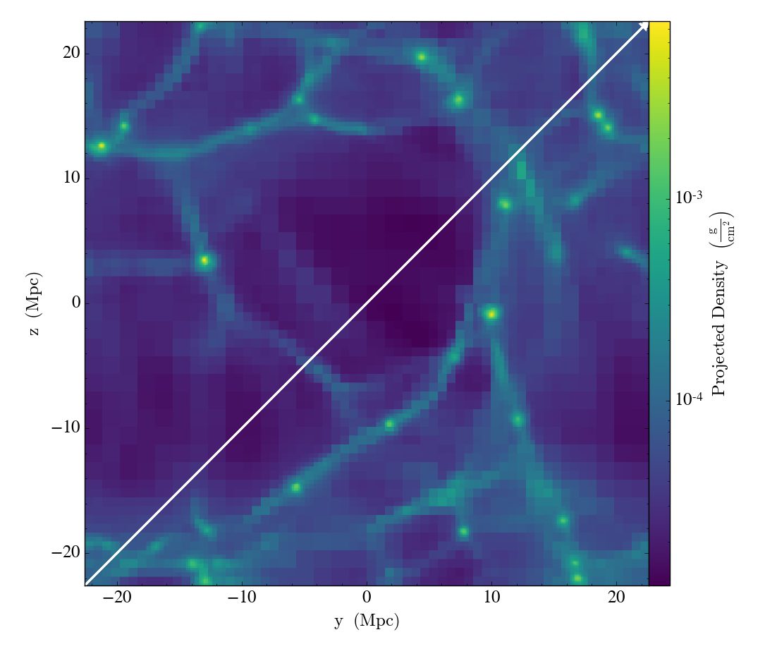
Overplotting a LightRay’s Trajectory on a Projection
Here we create a projection of the density field along the x axis of the
dataset, and then overplot the path the LightRay takes through the simulation,
before saving it to disk. The annotate_ray() operation should work for
any volumentric plot, including slices, and off-axis plots:
p = yt.ProjectionPlot(ds, 'x', 'density')
p.annotate_ray(ray, arrow=True)
p.save('projection.png')
Calculating Column Densities
Perhaps we wish to know the total column density of a particular ion present along
this LightRay. This can easily be done by multiplying the desired
ion number density field by the pathlength field, dl, to yield an array of
column densities for each resolution element, and then summing them together:
column_density_HI = ray.r[('gas', 'H_p0_number_density')] * ray.r[('gas', 'dl')]
print('HI Column Density = %g' % column_density_HI.sum())
Spectrum Generation
Now that we have our LightRay we can use it to generate a spectrum.
To create a spectrum, we need to make a SpectrumGenerator
object defining our desired wavelength range and bin size. You can do this
by manually setting these features, or just using one of the presets for
an instrument. Currently, we have three pre-defined instruments, the G130M,
G160M, and G140L observing modes for the Cosmic Origins Spectrograph aboard
the Hubble Space Telescope: COS-G130M, COS-G160M, and COS-G140L.
Notably, instrument COS aliases to COS-G130M.
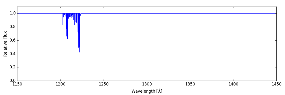
We then use this SpectrumGenerator object to make a raw
spectrum according to the intersecting fields it encountered in the
corresponding LightRay. We save this spectrum to disk, and
plot it:
sg = trident.SpectrumGenerator('COS-G130M')
sg.make_spectrum(ray, lines=line_list)
sg.save_spectrum('spec_raw.txt')
sg.plot_spectrum('spec_raw.png')
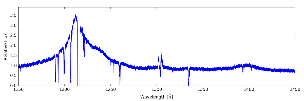
From here we can do some post-processing to the spectrum to include additional features that would be present in an actual observed spectrum. We add a background quasar spectrum, a Milky Way foreground, apply the COS line spread function, and add gaussian noise with SNR=30:
sg.add_qso_spectrum()
sg.add_milky_way_foreground()
sg.apply_lsf()
sg.add_gaussian_noise(30)
Finally, we use plot and save the resulting spectrum to disk:
sg.save_spectrum('spec_final.txt')
sg.plot_spectrum('spec_final.png')
which produces:
To create more complex or ion-specific spectra, refer to Advanced Spectrum Generation.
Compound LightRays
In some cases (e.g. studying redshift evolution of the IGM), it may be
desirable to create a LightRay that covers a range in redshift
that is larger than the domain width of a single simulation snaptshot.
Rather than simply sampling the same dataset repeatedly, which is
inherently unphysical since large scale structure evolves with cosmic
time, Trident allows the user to create a ray that samples multiple
datasets from different redshifts to produce a much longer ray that is
continuous in redshift space. This is done by using the
make_compound_ray() function. This function is
similar to the previously mentioned make_simple_ray()
function, but instead of accepting an individual dataset, it takes a
simulation parameter file, the associated simulation type, and the
desired range in redshift to be probed by the ray, while still
allowing the user to specify the same sort of line list as before::
fn = 'enzo_cosmology_plus/AMRCosmology.enzo'
ray = trident.make_compound_ray(fn, simulation_type='Enzo',
                                near_redshift=0.0, far_redshift=0.1,
                                lines=line_list)
In this example, we’ve created a ray from an Enzo simulation (the same one used above) that goes from z = 0 to z = 0.1. This ray can now be used to generate spectra in the exact same ways as before.
Obviously, there need to be sufficient simulation outputs over the desired
redshift range of the compound ray in order to have continuous sampling.
To assure adequate simulation output frequency for this, one can use yt’s
plan_cosmology_splice() function. See an example of its usage in
the yt_astro_analysis documentation.
We encourage you to look at the detailed documentation for
make_compound_ray() in the API Reference
section to understand how to control how the ray itself is constructed
from the available data.
Note
The compound ray functionality has only been implemented for the Enzo and Gadget simulation codes (and Gadget’s derivatives including Gizmo and AREPO). If you would like to help us implement this functionality for your simulation code, please contact us about this on the mailing list.